

Introduction
This software was developed to make full use of the data recorded by the Vector Vario in its enriched files (IGC+ format).
It enables highly detailed scientific flight analysis and in-depth discussion of the data and its interpretation.
This software was developed independently by Félix (a field operations engineer working in extreme environments).
He started this project during one of his recent missions in Antarctica, where he wrote the very first lines of code.
The different parts of the software:
Support
You can support Félix’s work and the future development of this software by buying him a coffee 😉
https://buymeacoffee.com/thegoodweather
Download
- Windows version: https://vectorvario.com/vva/VVA_v0.05_win.exe
- macOS version: https://vectorvario.com/vva/VVA_v0.05_mac.zip
Unzip the file, then move the app to the Applications folder. If macOS says the app cannot be opened, click Cancel, then go to System Settings → Privacy & Security → Security and click Open Anyway next to Vector Vario Analyzer. Sign in as an administrator, then confirm. - GitHub (source code): https://github.com/TheGoodWeather/Vector-Vario-Analyzer
Visit our updates page to see theversion history.
Questions
Félix develops this project in his spare time!
He and our team will do our best to answer questions, but we cannot provide full-time support.
Please use this Discord channel for your questions.
Importing flights
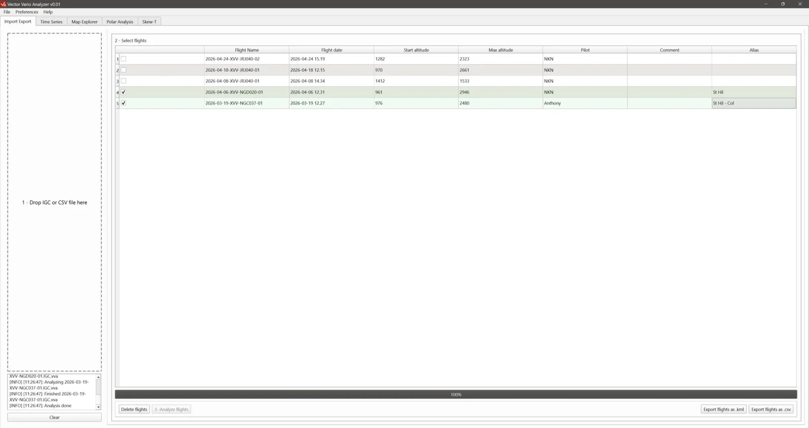
The first step is to import your files :
1 – Drag and drop your IGC files into the area on the left 1 – Drop IGC or CSV files here ;
2 – Successfully imported files are added to the list of flights already saved in the software, in the area 2 – Select flights;
3 – Click the button 3 – Analyze flights at the bottom of the window to analyse the selected flights. Once the import is complete, the other software tabs at the top of the window become available.
Notes:
- Successfully imported files are saved in a local software folder, together with all the settings changed while analysing each flight.
- In a new session, simply select flights already imported into the software (steps 2 and 3) to continue analysing them.
- If you analyse several flights at once, it is advisable to assign them an alias (last column in the table in the section 2 – Select flights). If an alias is defined, it replaces the filename as the flight identifier.
- From this tab, you can also export the selected flights in KML format (button Export flights as .kml) or CSV format (button Export flights as .csv) to continue your analysis in other software.
Time series
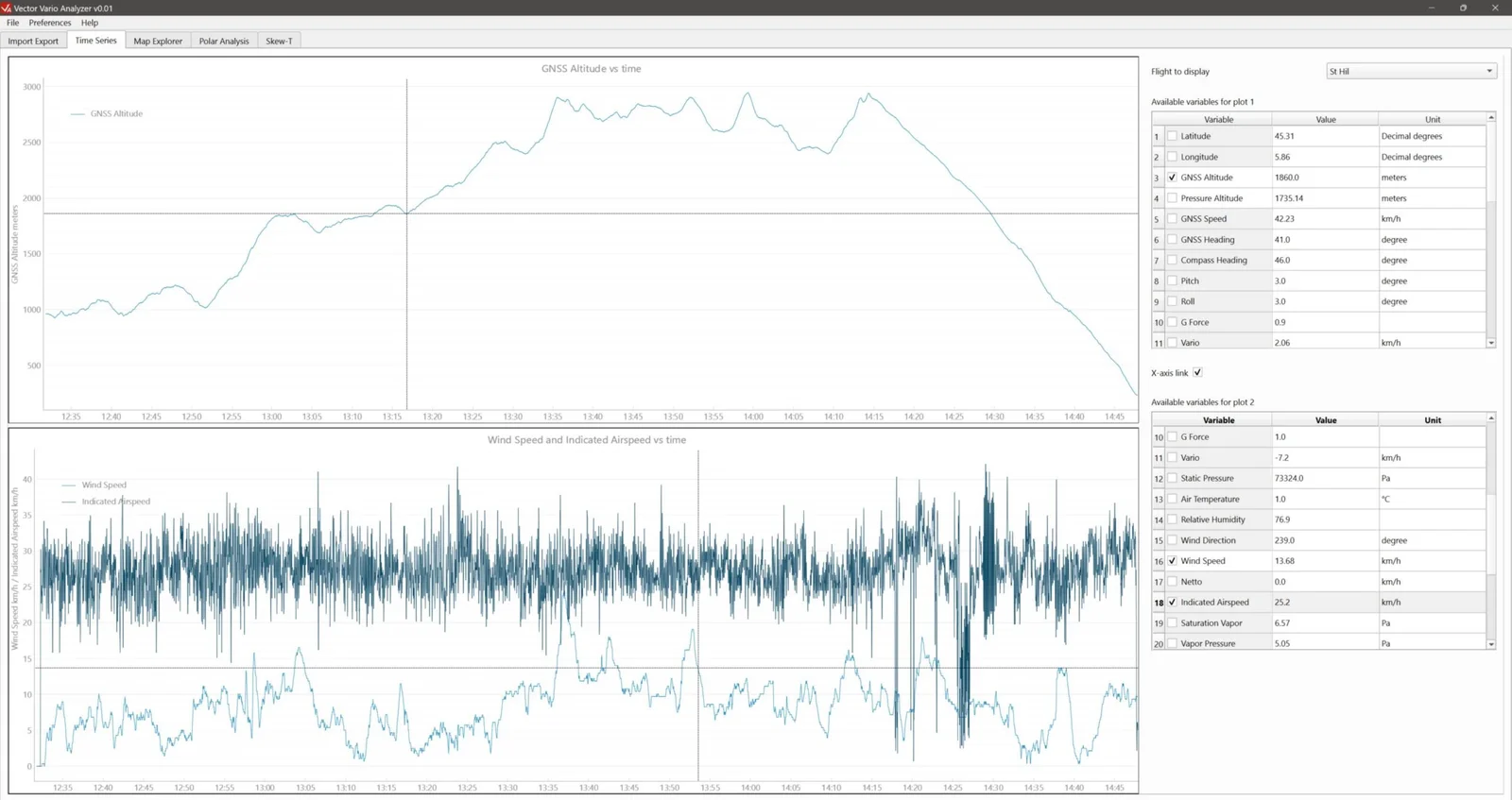
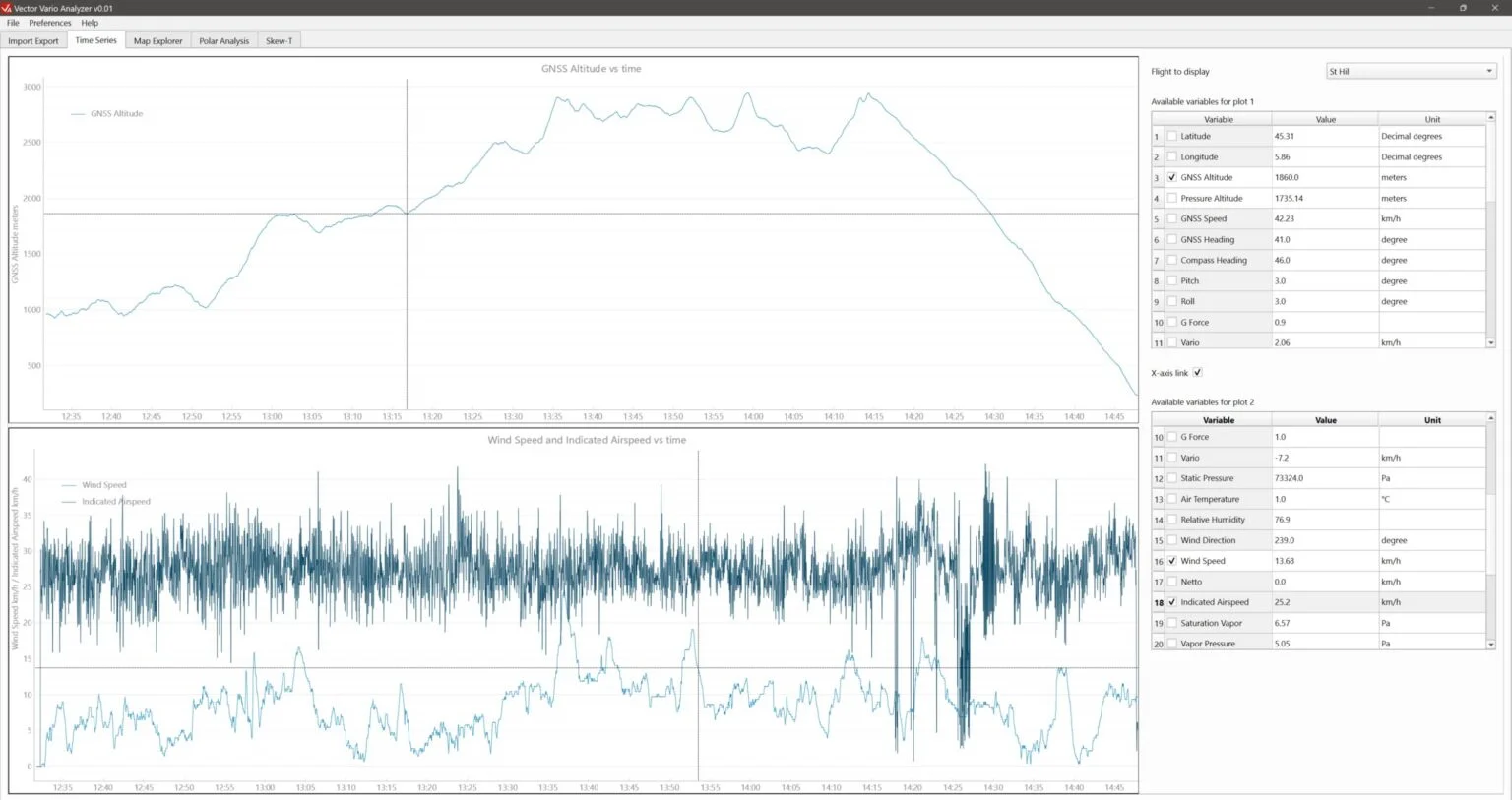
The Time Series tab lets you plot each parameter recorded in the IGC+ file.
Two separate plots (top and bottom) are available to display and compare different parameters:
- Select the flight from your imported flights in the drop-down list Flight to display, at the top right;
- Select the parameters to display in the tables Available variables for plot 1 and 2.
Notes:
- You can display several variables on the same graph, provided they have the same unit.
- To display simultaneously several variables with different units, use both graphs.
- The option X-axis link between the two tables synchronises the X-axis (time) of the two plots.
- The units can be changed in the menu Preferences > Units.
Available parameters
Parameters recorded directly in the IGC+ file:
- Latitude
- Longitude
- GNSS altitude
- Pressure altitude
- Heading (compass)
- Pitch
- Roll
- Load factor (G)
- Air temperature
- Relative air humidity
- Wind direction
- Wind speed
- Netto
- IAS (Indicated Airspeed)
Parameters calculated from the original parameters:
- GNSS speed
- GNSS heading
- Vario
- Static pressure
- Saturation vapour pressure
- Vapour pressure
- Mixing ratio
- Dew-point temperature
- Cloud-base altitude
- Potential temperature
- Air density
- IAS vario
- TAS (True Airspeed)
Mouse controls
- Left click: move the graph.
- Right click and drag (up/down or left/right): zoom independently on the X- or Y-axis.
- Scroll wheel: zoom in/out.
- Click a point on the curve: display detailed information about that point in the tables on the right.
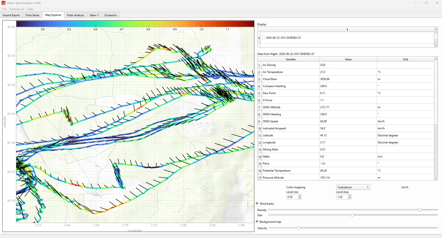
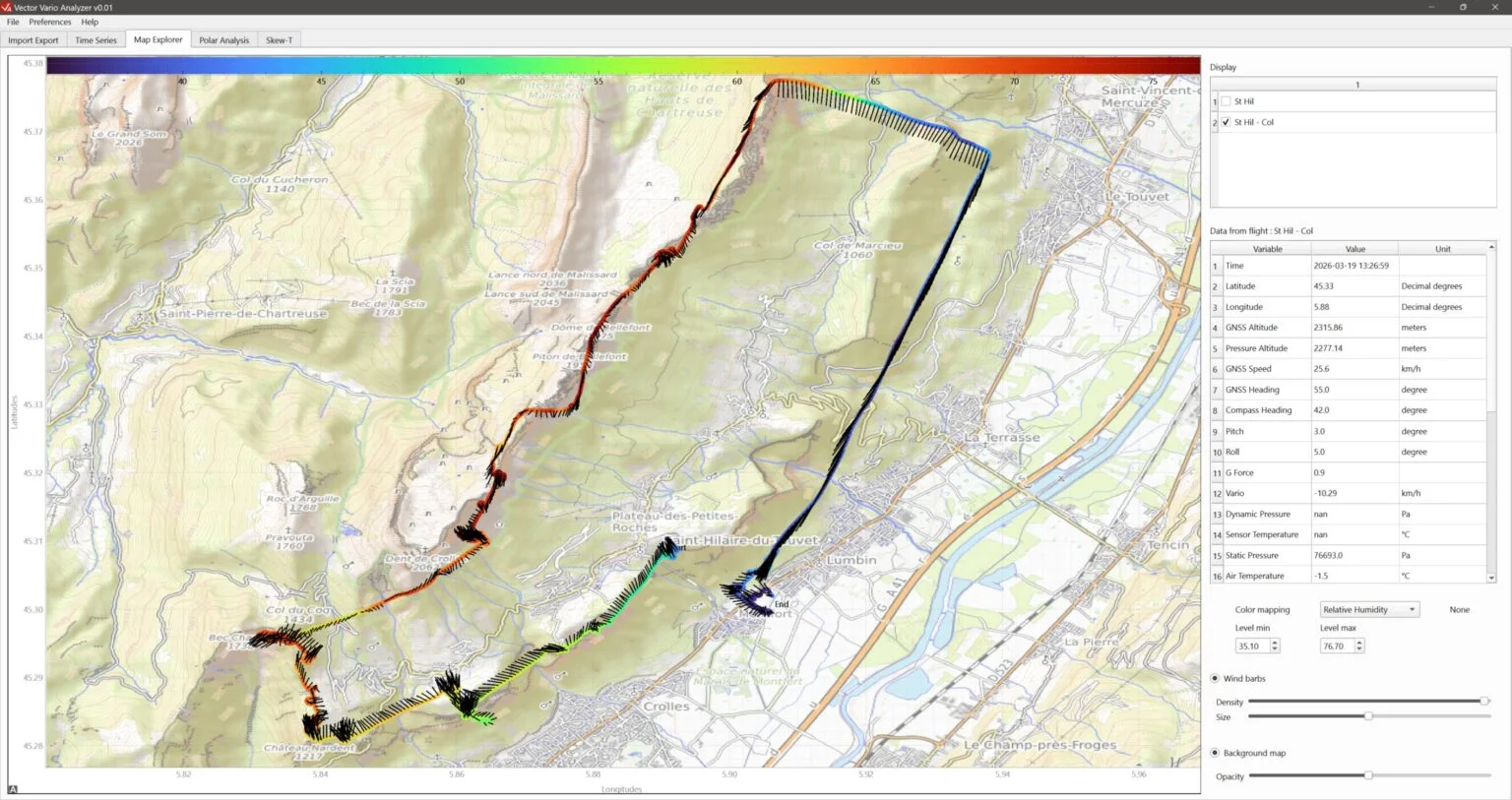
Map view
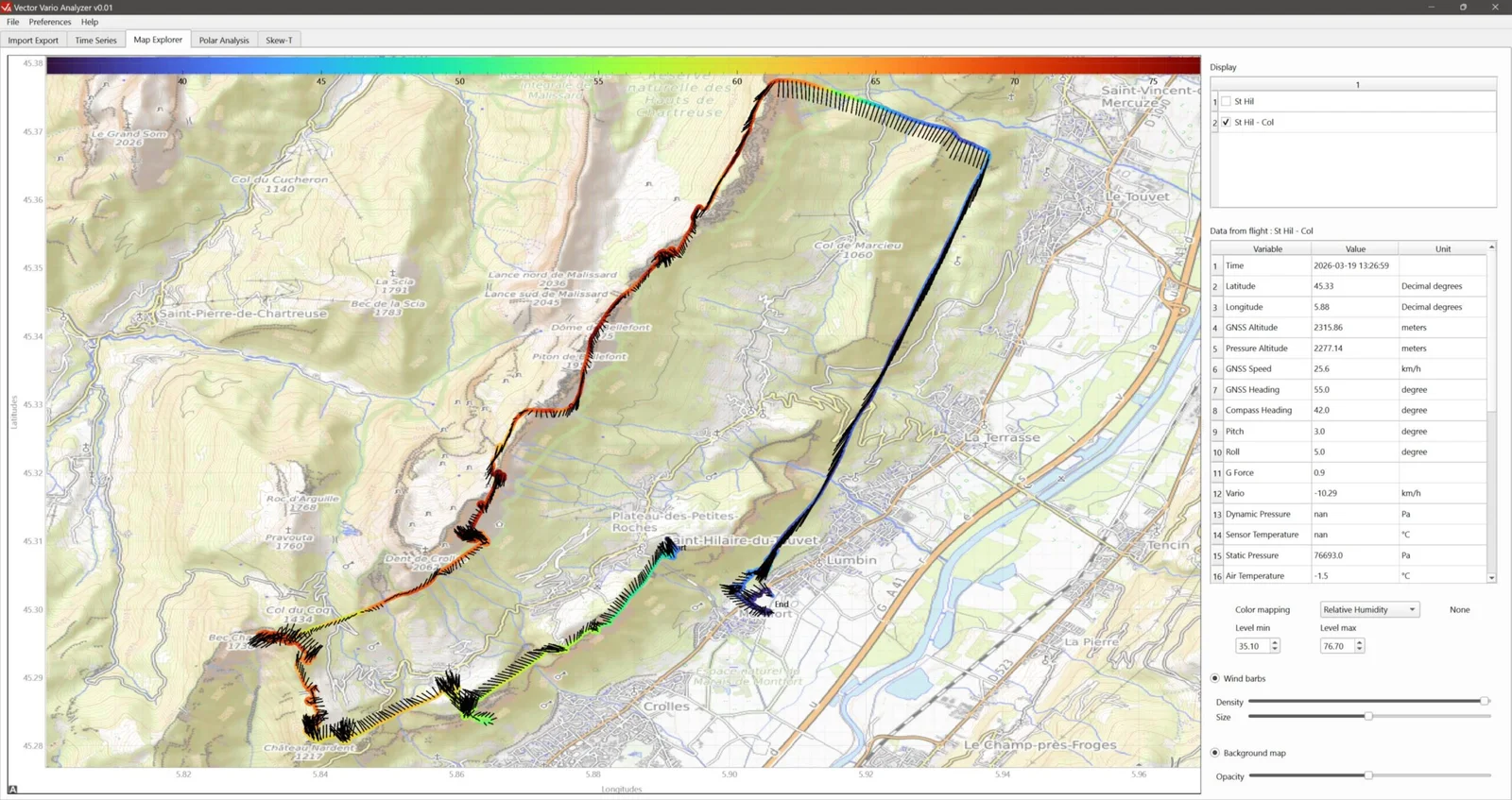
To display data on a map:
- Select the flights to display simultaneously in the list at the top right (Display);
- Optionally, in the drop-down list Colour mapping select the variable used to colour the displayed tracks. You can change the colour-scale limits by adjusting the values Level min and Level max.
- Optionally, add wind barbs to the displayed tracks by selecting Wind barbs. Their density and size can be adjusted with the sliders Density and Size. Note that the wind barbs here behave like wool threads carried by the wind, rather than showing where the wind comes from.
- Optionally, show or hide the background map (Background Map).
Notes:
- Clicking a point on the track displays the value of each variable at that point in the table on the right.
- An internet connection is required to load the background map (OpenStreetMap).
Mouse controls
- Left click and drag: move the map.
- Scroll wheel: zoom.
- Right click and drag up/down: zoom.
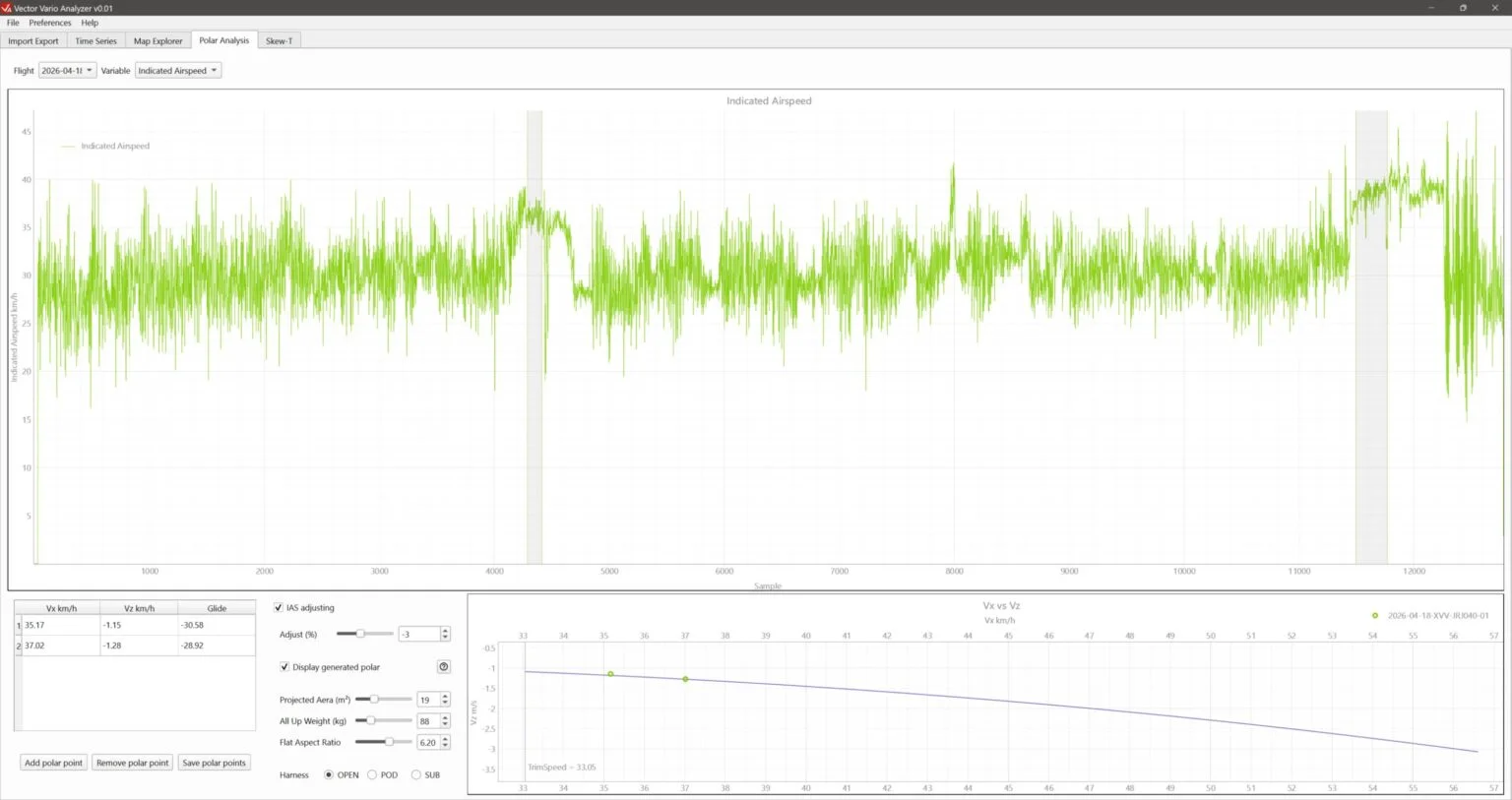
Speed polar
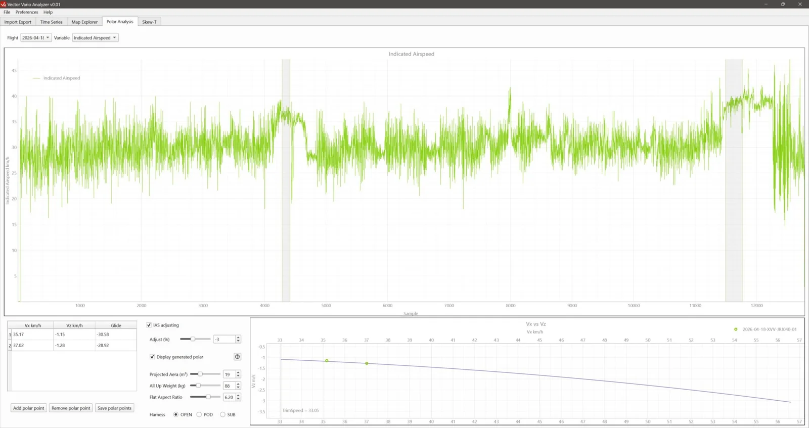
In flight:
- Fly in stable conditions with no wind;
- Maintain a given flight regime (hands up, accelerated or with brake input) for more than 20 seconds.
- Keep the pilot’s position identical and use the same harness between measurements (within one flight and between flights) so that the data can be compared meaningfully.
To analyse the data:
- Select the flight to display from your imported flights (drop-down menu Flights).
- Select the variable GNSS Altitude (default) or IAS (Indicated Airspeed) to display in the upper graph. Use this graph to identify the flight regimes you want to study.
- Click add a point (Add polar point) at the bottom left of the window. This adds a shaded area to the graph that you can move and adjust. The airspeed (Vx) and vario (Vz) data in this area are averaged into a point, which is added to the table at the bottom left and the graph at the bottom right.
- Repeat the selection for the other points.
- Add the theoretical speed polar to the bottom-right graph by selecting Display generated polar.
- Enter the theoretical parameters as configured on your Vector Vario to plot the curve used in flight.
Mouse controls
- Usual controls for this type of graph.
- Left click and drag a selection area: move the area.
- Left click and drag an edge of a selection area: move that edge.
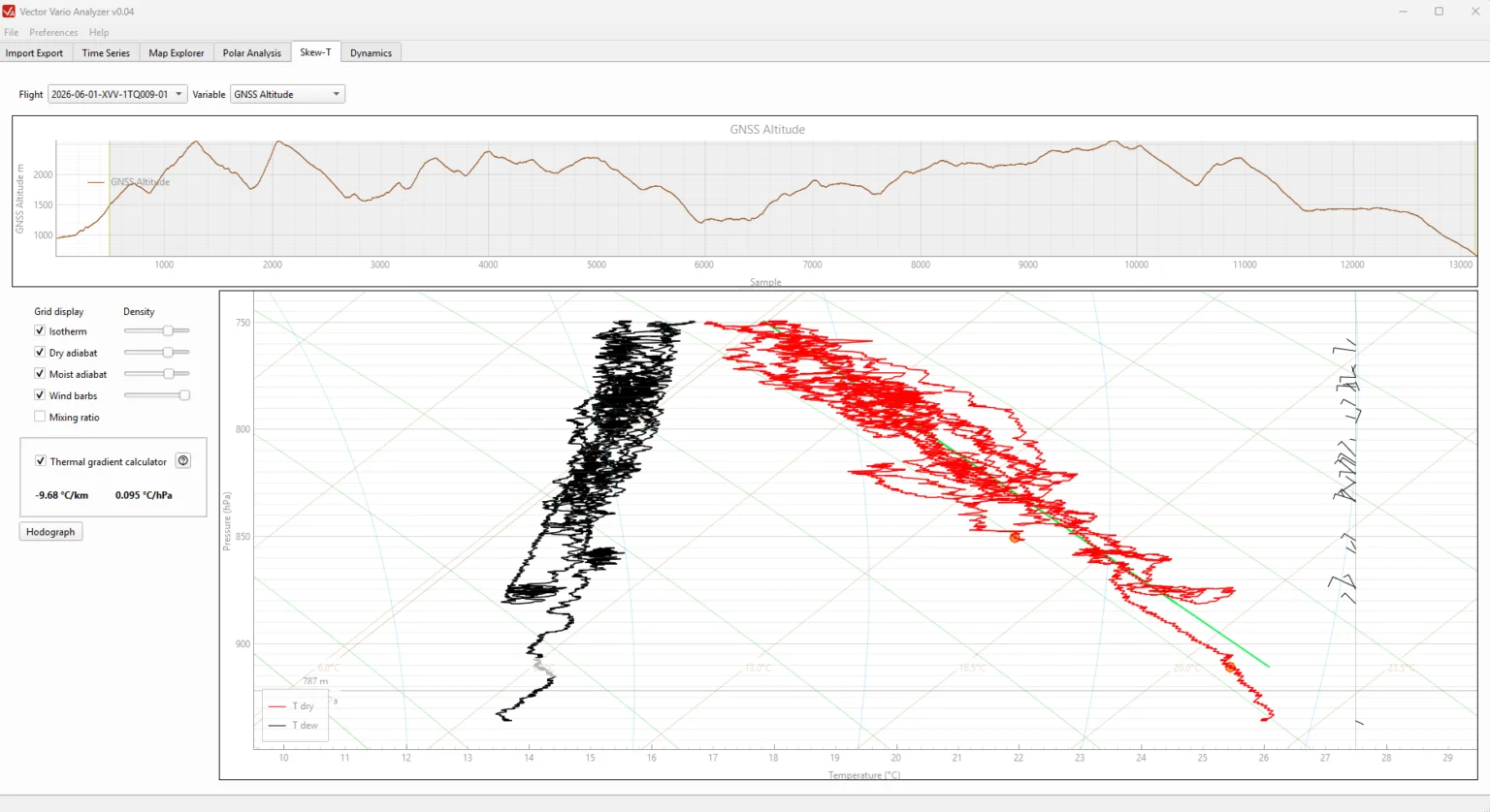
Skew-T diagram
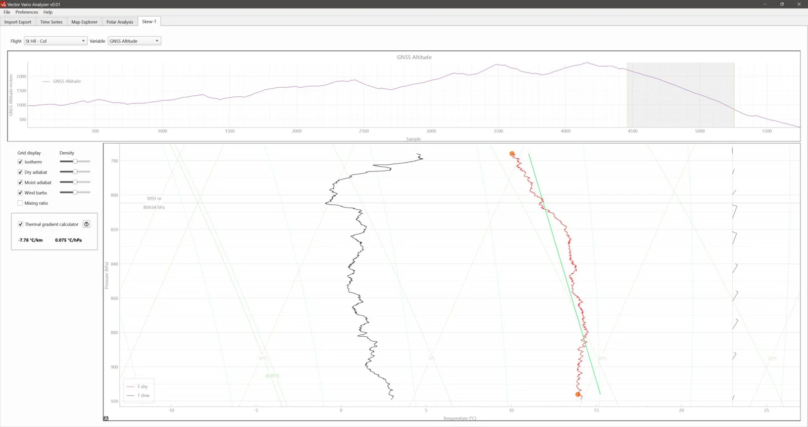
- Select the flight from the imported flights (drop-down menu Flights).
- Select the variable to display in the upper graph. This graph helps you select the data range of interest. It can display any of the available variables.
- Move and adjust the selection area (shaded area), which defines the flight data displayed on the Skew-T diagram.
- Optionally, enable the thermal gradient calculator (Thermal gradient calulator), which calculates the temperature gradient between two movable points on the temperature profile. The colour of the line connecting them indicates atmospheric stability.
Notes:
- Keep the spatial and temporal nature of the data in mind, and consider whether it is appropriate to combine measurements taken at different times and/or in different locations.
- The data may also combine measurements from adiabatic conditions (for example, when passing through a thermal) with measurements of the surrounding atmosphere.
Mouse controls
- Usual controls for this type of graph.
- Left click and drag a selection area: move the area.
- Left click and drag an edge of a selection area: move that edge.
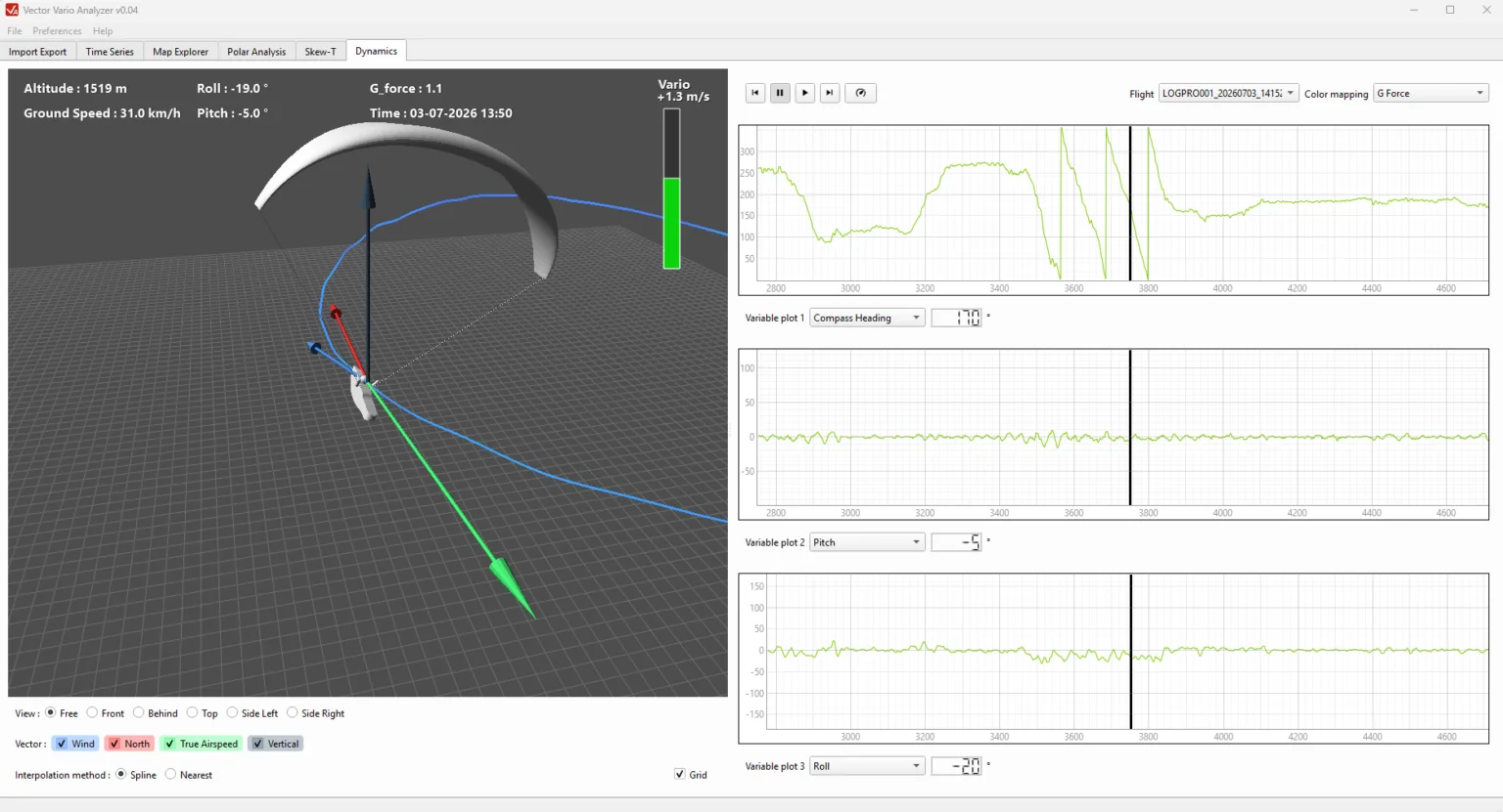
Flight dynamics
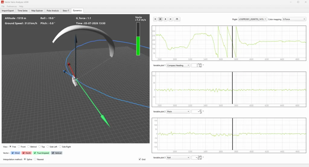
- Select the flight from the imported flights (drop-down menu Flights).
- Select the variable to display in colour (G-force by default). This graph can display any of the available variables.
- To start the animation, click the button Play. Playback speed can be changed using the speed selector.
- By default, heading, pitch and roll are displayed as graphs on the right of the window. A black cursor indicates the playback position.
- In the 3D view, the default display mode is Free. Use the mouse to change the viewing angle (left click) and zoom level (scroll wheel). The camera stays centred on the paraglider. You can also select a fixed viewpoint using the buttons below the window.
- Optionally, display the vectors for wind, airspeed, north and vertical by selecting the boxes at the bottom of the window.
- The default interpolation type is Spline, which produces smooth animation. To view the raw data exactly as recorded in the IGC file, select Nearest, which uses the exact recorded values.
Note:
Reconstructing a paraglider flight in 3D is complex. This visualisation is still experimental and may contain inaccuracies, particularly outside the normal flight envelope or during manoeuvres with a high load factor.
Mouse controls
- Left click in the 3D view: change the camera angle
- Scroll wheel in the 3D view: change the camera zoom
- Left click on the 1D plots: move the playback cursor
- 1D plots: Usual controls for this type of graph.